Faceted search is as crucial to a modern search application as autocomplete, spell correction, and search keywords highlighting, especially in e-commerce products.
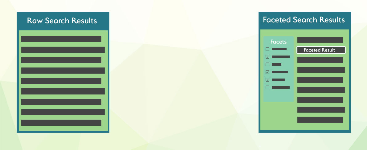
Faceted search comes in handy when dealing with large quantities of data and various interconnected properties, such as size, color, manufacturer, or other factors. When querying vast amounts of data, search results frequently include numerous entries that don't match the user's expectations. Faceted search enables the end user to explicitly define the criteria they want their search results to satisfy.
In Manticore Search, there's an optimization that maintains the result set of the original query and reuses it for each facet calculation. Since the aggregations are applied to an already calculated subset of documents, they're fast, and the total execution time can often be only slightly longer than the initial query. Facets can be added to any query, and the facet can be any attribute or expression. A facet result includes the facet values and the facet counts. Facets can be accessed using the SQL SELECT statement by declaring them at the very end of the query.
The facet values can originate from an attribute, a JSON property within a JSON attribute, or an expression. Facet values can also be aliased, but the alias must be unique across all result sets (main query result set and other facets result sets). The facet value is derived from the aggregated attribute/expression, but it can also come from another attribute/expression.
FACET {expr_list} [BY {expr_list}] [ALL FILTERS | FILTERS {expr_list} | EXCLUDE FILTERS {expr_list}] [ZEROES] [MODE {strict | auto | max}] [DISTINCT {field_name}] [ORDER BY {expr | FACET()} {ASC | DESC}] [LIMIT [offset,] count]Multiple facet declarations must be separated by a whitespace.
Facets can be defined in the aggs node:
     "aggs" :
     {
        "group name" :
         {
            "terms" :
             {
              "field":"attribute name",
              "size": 1000
             }
             "sort": [ {"attribute name": { "order":"asc" }} ]
         }
     }
where:
group nameis an alias assigned to the aggregationfieldvalue must contain the name of the attribute or expression being faceted- optional
sizespecifies the maximum number of buckets to include in the result. When not specified, it inherits the main query's limit. More details can be found in the Size of facet result section. - optional
sortspecifies an array of attributes and/or additional properties using the same syntax as the "sort" parameter in the main query. - optional top-level
facet_filter_modecontrols how all aggregations inherit filters from the main query. Supported values arestrict,auto, andmax. This is the query-level setting in SQL (OPTION facet_filter_mode='...') and the top-level setting in JSON. - optional per-aggregation
modeoverrides the inherited mode for that aggregation. Supported values arestrict,auto, andmax. This key is JSON-only and is not an alias forfacet_filter_mode. In SQL, the equivalent per-facet override is theMODEkeyword inside aFACETclause. - optional per-aggregation
filtersexplicitly lists which main-query attribute filters should be applied to that aggregation. In SQL the equivalent clause isFILTERS .... - optional per-aggregation
exclude_filtersexplicitly lists which main-query attribute filters should not be applied to that aggregation. This key is JSON-only; in SQL the equivalent clause isEXCLUDE FILTERS .... - optional per-aggregation
zeroesenables zero-count buckets inmaxmode. In SQL, the equivalent per-facet keyword isZEROES. If you want filtered visible counts in SQLmaxmode and also want broad zero-count buckets, useOPTION facet_filter_mode='max' ... FACET ... ALL FILTERS ZEROES. autoandmaxfacet result sets can include astatusbucket marker. Returned values areselected,available, andunavailable.
The result set will contain an aggregations node with the returned facets, where key is the aggregated value and doc_count is the aggregation count.
    "aggregations": {
        "group name": {
        "buckets": [
            {
                "key": 10,
                "doc_count": 1019
            },
            {
                "key": 9,
                "doc_count": 954
            },
            {
                "key": 8,
                "doc_count": 1021
            },
            {
                "key": 7,
                "doc_count": 1011
            },
            {
                "key": 6,
                "doc_count": 997
            }
            ]
        }
}- SQL
- JSON
- PHP
- Python
- Python-asyncio
- Javascript
- Java
- C#
- Rust
- TypeScript
- Go
SELECT *, price AS aprice FROM facetdemo LIMIT 10 FACET price LIMIT 10 FACET brand_id LIMIT 5;+------+-------+----------+---------------------+------------+-------------+---------------------------------------+------------+--------+
| id | price | brand_id | title | brand_name | property | j | categories | aprice |
+------+-------+----------+---------------------+------------+-------------+---------------------------------------+------------+--------+
| 1 | 306 | 1 | Product Ten Three | Brand One | Six_Ten | {"prop1":66,"prop2":91,"prop3":"One"} | 10,11 | 306 |
| 2 | 400 | 10 | Product Three One | Brand Ten | Four_Three | {"prop1":69,"prop2":19,"prop3":"One"} | 13,14 | 400 |
...
| 9 | 560 | 6 | Product Two Five | Brand Six | Eight_Two | {"prop1":90,"prop2":84,"prop3":"One"} | 13,14 | 560 |
| 10 | 229 | 9 | Product Three Eight | Brand Nine | Seven_Three | {"prop1":84,"prop2":39,"prop3":"One"} | 12,13 | 229 |
+------+-------+----------+---------------------+------------+-------------+---------------------------------------+------------+--------+
10 rows in set (0.00 sec)
+-------+----------+
| price | count(*) |
+-------+----------+
| 306 | 7 |
| 400 | 13 |
...
| 229 | 9 |
| 595 | 10 |
+-------+----------+
10 rows in set (0.00 sec)
+----------+----------+
| brand_id | count(*) |
+----------+----------+
| 1 | 1013 |
| 10 | 998 |
| 5 | 1007 |
| 8 | 1033 |
| 7 | 965 |
+----------+----------+
5 rows in set (0.00 sec)Data can be faceted by aggregating another attribute or expression. For example if the documents contain both the brand id and name, we can return in facet the brand names, but aggregate the brand ids. This can be done by using FACET {expr1} BY {expr2}
- SQL
- JSON
SELECT * FROM facetdemo FACET brand_name by brand_id;+------+-------+----------+---------------------+-------------+-------------+---------------------------------------+------------+
| id | price | brand_id | title | brand_name | property | j | categories |
+------+-------+----------+---------------------+-------------+-------------+---------------------------------------+------------+
| 1 | 306 | 1 | Product Ten Three | Brand One | Six_Ten | {"prop1":66,"prop2":91,"prop3":"One"} | 10,11 |
| 2 | 400 | 10 | Product Three One | Brand Ten | Four_Three | {"prop1":69,"prop2":19,"prop3":"One"} | 13,14 |
....
| 19 | 855 | 1 | Product Seven Two | Brand One | Eight_Seven | {"prop1":63,"prop2":78,"prop3":"One"} | 10,11,12 |
| 20 | 31 | 9 | Product Four One | Brand Nine | Ten_Four | {"prop1":79,"prop2":42,"prop3":"One"} | 12,13,14 |
+------+-------+----------+---------------------+-------------+-------------+---------------------------------------+------------+
20 rows in set (0.00 sec)
+-------------+----------+
| brand_name | count(*) |
+-------------+----------+
| Brand One | 1013 |
| Brand Ten | 998 |
| Brand Five | 1007 |
| Brand Nine | 944 |
| Brand Two | 990 |
| Brand Six | 1039 |
| Brand Three | 1016 |
| Brand Four | 994 |
| Brand Eight | 1033 |
| Brand Seven | 965 |
+-------------+----------+
10 rows in set (0.00 sec)If you need to remove duplicates from the buckets returned by FACET, you can use DISTINCT field_name, where field_name is the field by which you want to perform deduplication. It can also be id (which is the default) if you make a FACET query against a distributed table and are not sure whether you have unique ids in the tables (the tables should be local and have the same schema).
If you have multiple FACET declarations in your query, field_name should be the same in all of them.
DISTINCT returns an additional column count(distinct ...) before the column count(*), allowing you to obtain both results without needing to make another query.
- SQL
- JSON
SELECT brand_name, property FROM facetdemo FACET brand_name distinct property;+-------------+----------+
| brand_name | property |
+-------------+----------+
| Brand Nine | Four |
| Brand Ten | Four |
| Brand One | Five |
| Brand Seven | Nine |
| Brand Seven | Seven |
| Brand Three | Seven |
| Brand Nine | Five |
| Brand Three | Eight |
| Brand Two | Eight |
| Brand Six | Eight |
| Brand Ten | Four |
| Brand Ten | Two |
| Brand Four | Ten |
| Brand One | Nine |
| Brand Four | Eight |
| Brand Nine | Seven |
| Brand Four | Five |
| Brand Three | Four |
| Brand Four | Two |
| Brand Four | Eight |
+-------------+----------+
20 rows in set (0.00 sec)
+-------------+--------------------------+----------+
| brand_name | count(distinct property) | count(*) |
+-------------+--------------------------+----------+
| Brand Nine | 3 | 3 |
| Brand Ten | 2 | 3 |
| Brand One | 2 | 2 |
| Brand Seven | 2 | 2 |
| Brand Three | 3 | 3 |
| Brand Two | 1 | 1 |
| Brand Six | 1 | 1 |
| Brand Four | 4 | 5 |
+-------------+--------------------------+----------+
8 rows in set (0.00 sec)Facets can aggregate over expressions. A classic example is the segmentation of prices by specific ranges:
- SQL
- JSON
- PHP
- Python
- Python-asyncio
- Javascript
- Java
- C#
- Rust
- TypeScript
- Go
SELECT * FROM facetdemo FACET INTERVAL(price,200,400,600,800) AS price_range ;+------+-------+----------+---------------------+-------------+-------------+---------------------------------------+------------+-------------+
| id | price | brand_id | title | brand_name | property | j | categories | price_range |
+------+-------+----------+---------------------+-------------+-------------+---------------------------------------+------------+-------------+
| 1 | 306 | 1 | Product Ten Three | Brand One | Six_Ten | {"prop1":66,"prop2":91,"prop3":"One"} | 10,11 | 1 |
...
+------+-------+----------+---------------------+-------------+-------------+---------------------------------------+------------+-------------+
20 rows in set (0.00 sec)
+-------------+----------+
| price_range | count(*) |
+-------------+----------+
| 0 | 1885 |
| 3 | 1973 |
| 4 | 2100 |
| 2 | 1999 |
| 1 | 2043 |
+-------------+----------+
5 rows in set (0.01 sec)Facets can aggregate over multi-level grouping, with the result set being the same as if the query performed a multi-level grouping:
- SQL
- JSON
SELECT *,INTERVAL(price,200,400,600,800) AS price_range FROM facetdemo
FACET price_range AS price_range,brand_name ORDER BY brand_name asc;+------+-------+----------+---------------------+-------------+-------------+---------------------------------------+------------+-------------+
| id | price | brand_id | title | brand_name | property | j | categories | price_range |
+------+-------+----------+---------------------+-------------+-------------+---------------------------------------+------------+-------------+
| 1 | 306 | 1 | Product Ten Three | Brand One | Six_Ten | {"prop1":66,"prop2":91,"prop3":"One"} | 10,11 | 1 |
...
+------+-------+----------+---------------------+-------------+-------------+---------------------------------------+------------+-------------+
20 rows in set (0.00 sec)
+--------------+-------------+----------+
| fprice_range | brand_name | count(*) |
+--------------+-------------+----------+
| 1 | Brand Eight | 197 |
| 4 | Brand Eight | 235 |
| 3 | Brand Eight | 203 |
| 2 | Brand Eight | 201 |
| 0 | Brand Eight | 197 |
| 4 | Brand Five | 230 |
| 2 | Brand Five | 197 |
| 1 | Brand Five | 204 |
| 3 | Brand Five | 193 |
| 0 | Brand Five | 183 |
| 1 | Brand Four | 195 |
...Facets can aggregate over histogram values by constructing fixed-size buckets over the values. The key function is:
key_of_the_bucket = interval + offset * floor ( ( value - offset ) / interval )The histogram argument interval must be positive, and the histogram argument offset must be positive and less than interval. By default, the buckets are returned as an array. The histogram argument keyed makes the response a dictionary with the bucket keys.
- SQL
- JSON
- JSON 2
SELECT COUNT(*), HISTOGRAM(price, {hist_interval=100}) as price_range FROM facets GROUP BY price_range ORDER BY price_range ASC;+----------+-------------+
| count(*) | price_range |
+----------+-------------+
| 5 | 0 |
| 5 | 100 |
| 1 | 300 |
| 4 | 400 |
| 1 | 500 |
| 3 | 700 |
| 1 | 900 |
+----------+-------------+Facets can aggregate over histogram date values, which is similar to the normal histogram. The difference is that the interval is specified using a date or time expression. Such expressions require special support because the intervals are not always of fixed length. Values are rounded to the closest bucket using the following key function:
key_of_the_bucket = interval * floor ( value / interval )The histogram parameter calendar_interval understands months to have different amounts of days.
Unlike calendar_interval, the fixed_interval parameter uses a fixed number of units and does not deviate, regardless of where it falls on the calendar. However fixed_interval cannot process units such as months because a month is not a fixed quantity. Attempting to specify units like weeks or months for fixed_interval will result in an error.
The accepted intervals are described in the date_histogram expression. By default, the buckets are returned as an array. The histogram argument keyed makes the response a dictionary with the bucket keys.
In JSON queries, date_histogram also supports time_zone and offset with calendar_interval:
time_zonechanges the timezone used to round calendar buckets and to formatkey_as_string. It must be an IANA timezone name supported by the server, for exampleAsia/Novosibirsk. Numeric UTC offsets such as+03:00are not supported.offsetshifts calendar bucket boundaries by a fixed amount before rounding. It can be a fixed-interval string using the same units asfixed_interval, for example3h, or an integer number of seconds, for example10800. The value can be prefixed with+or-.
time_zone and offset are not supported with fixed_interval.
- SQL
- JSON
SELECT count(*), DATE_HISTOGRAM(tm, {calendar_interval='month'}) AS months FROM idx_dates GROUP BY months ORDER BY months ASC+----------+------------+
| count(*) | months |
+----------+------------+
| 442 | 1485907200 |
| 744 | 1488326400 |
| 720 | 1491004800 |
| 230 | 1493596800 |
+----------+------------+Facets can aggregate over a set of ranges. The values are checked against the bucket range, where each bucket includes the from value and excludes the to value from the range.
Setting the keyed property to true makes the response a dictionary with the bucket keys rather than an array.
- SQL
- JSON
- JSON 2
SELECT COUNT(*), RANGE(price, {range_to=150},{range_from=150,range_to=300},{range_from=300}) price_range FROM facets GROUP BY price_range ORDER BY price_range ASC;+----------+-------------+
| count(*) | price_range |
+----------+-------------+
| 8 | 0 |
| 2 | 1 |
| 10 | 2 |
+----------+-------------+Facets can aggregate over a set of date ranges, which is similar to the normal range. The difference is that the from and to values can be expressed in Date math expressions. This aggregation includes the from value and excludes the to value for each range. Setting the keyed property to true makes the response a dictionary with the bucket keys rather than an array.
- SQL
- JSON
SELECT COUNT(*), DATE_RANGE(tm, {range_to='2017||+2M/M'},{range_from='2017||+2M/M',range_to='2017||+5M/M'},{range_from='2017||+5M/M'}) AS points FROM idx_dates GROUP BY points ORDER BY points ASC;+----------+--------+
| count(*) | points |
+----------+--------+
| 442 | 0 |
| 1464 | 1 |
| 230 | 2 |
+----------+--------+Facets support the ORDER BY clause just like a standard query. Each facet can have its own ordering, and the facet ordering doesn't affect the main result set's ordering, which is determined by the main query's ORDER BY. Sorting can be done on attribute name, count (using COUNT(*), COUNT(DISTINCT attribute_name)), or the special FACET() function, which provides the aggregated data values. By default, a query with ORDER BY COUNT(*) will sort in descending order.
- SQL
- JSON
SELECT * FROM facetdemo
FACET brand_name BY brand_id ORDER BY FACET() ASC
FACET brand_name BY brand_id ORDER BY brand_name ASC
FACET brand_name BY brand_id order BY COUNT(*) DESC;
FACET brand_name BY brand_id order BY COUNT(*);+------+-------+----------+---------------------+-------------+-------------+---------------------------------------+------------+
| id | price | brand_id | title | brand_name | property | j | categories |
+------+-------+----------+---------------------+-------------+-------------+---------------------------------------+------------+
| 1 | 306 | 1 | Product Ten Three | Brand One | Six_Ten | {"prop1":66,"prop2":91,"prop3":"One"} | 10,11 |
...
| 20 | 31 | 9 | Product Four One | Brand Nine | Ten_Four | {"prop1":79,"prop2":42,"prop3":"One"} | 12,13,14 |
+------+-------+----------+---------------------+-------------+-------------+---------------------------------------+------------+
20 rows in set (0.01 sec)
+-------------+----------+
| brand_name | count(*) |
+-------------+----------+
| Brand One | 1013 |
| Brand Two | 990 |
| Brand Three | 1016 |
| Brand Four | 994 |
| Brand Five | 1007 |
| Brand Six | 1039 |
| Brand Seven | 965 |
| Brand Eight | 1033 |
| Brand Nine | 944 |
| Brand Ten | 998 |
+-------------+----------+
10 rows in set (0.01 sec)
+-------------+----------+
| brand_name | count(*) |
+-------------+----------+
| Brand Eight | 1033 |
| Brand Five | 1007 |
| Brand Four | 994 |
| Brand Nine | 944 |
| Brand One | 1013 |
| Brand Seven | 965 |
| Brand Six | 1039 |
| Brand Ten | 998 |
| Brand Three | 1016 |
| Brand Two | 990 |
+-------------+----------+
10 rows in set (0.01 sec)
+-------------+----------+
| brand_name | count(*) |
+-------------+----------+
| Brand Six | 1039 |
| Brand Eight | 1033 |
| Brand Three | 1016 |
| Brand One | 1013 |
| Brand Five | 1007 |
| Brand Ten | 998 |
| Brand Four | 994 |
| Brand Two | 990 |
| Brand Seven | 965 |
| Brand Nine | 944 |
+-------------+----------+
10 rows in set (0.01 sec)Before counting buckets for a facet, Manticore first decides which filters from the main query should be applied to that facet.
Built-in modes:
strict- apply all filters from the main query and keep regular facet output
auto- apply all filters from the main query except filters on this same facet
- add a
statusmarker; selected buckets areselected, sibling buckets areavailable
max- count buckets from the broad base query and add a
statusmarker for each bucket
- count buckets from the broad base query and add a
Manual overrides:
- SQL
ALL FILTERS- apply all main-query filters to this facet
- SQL
FILTERS .../ JSONfilters- apply only the listed main-query filters to this facet
- SQL
EXCLUDE FILTERS .../ JSONexclude_filters- apply all main-query filters except the listed ones to this facet
Short version:
strict= apply everythingauto= apply everything except this facet's own filters +statusmax= broad base-query counts +status- SQL
ALL FILTERS= apply everything - SQL
FILTERS= apply only these filters - JSON
exclude_filters/ SQLEXCLUDE FILTERS= apply everything except these filters
Performance note:
maxis the most expensive facet mode because it has to collect broad facet counts and strict/current availability metadata- on large datasets or queries with many facets,
maxcan be much slower thanstrictorauto - use
autowhen the UI needs selectable buckets from the current filter scope, andmaxwhen it also needs broad bucket lists with unavailable values
Example
If the main query has:
brand='nike'color='red'size='small'
and we calculate FACET color, then:
strict- apply
brand + color + size
- apply
auto- apply
brand + size - and return selected color buckets with
status=selectedand sibling color buckets withstatus=available
- apply
max- apply the broad base query without
brand,color, orsize - and return color buckets with
status
- apply the broad base query without
filters=["brand"]- apply only
brand
- apply only
exclude_filters=["size"]- apply
brand + color
- apply
- SQL
- JSON
SELECT id
FROM products
WHERE MATCH('sneakers') AND color_id=1 AND size_id=42 AND brand_id=7
OPTION facet_filter_mode='max'
FACET color_id ALL FILTERS
FACET size_id
FACET sku FILTERS color_id, size_id
FACET brand_id EXCLUDE FILTERS color_id;
The per-facet SQL clauses mean:
ALL FILTERS— apply all main-query filters to this facetFILTERS color_id, size_id— apply onlycolor_idandsize_idfilters to this facetEXCLUDE FILTERS color_id— apply all main-query filters exceptcolor_idto this facetMODE max— override the inherited facet mode for this one SQL facetZEROES— in SQLmaxmode, keep buckets from the broadermaxbucket universe even when the visible facet count is0; in JSON the equivalent per-aggregation key is"zeroes": true
The naming differs slightly between SQL and JSON:
- SQL uses the query option
facet_filter_mode, the per-facet keywordMODE, and the clausesFILTERS/EXCLUDE FILTERS - JSON uses the top-level key
facet_filter_mode, the per-aggregation keysmode/zeroes, and the keysfilters/exclude_filters
There is no query-level mode key. Use facet_filter_mode for the inherited query/top-level default, MODE for one SQL facet, and mode for one JSON aggregation.
ZEROES does not replace MODE max; it works with max mode. So if the query already has OPTION facet_filter_mode='max', the SQL form is simply FACET color_id ALL FILTERS ZEROES. If the query default stays strict or auto, enable max on that one facet explicitly with FACET color_id ALL FILTERS ZEROES MODE max.
These clauses override the filter scope that would otherwise come from facet_filter_mode or SQL MODE. For example, with OPTION facet_filter_mode='max', FACET color_id ALL FILTERS ZEROES still emits status, its visible counts use all main-query filters, and ZEROES keeps broad max buckets that are missing from the filtered counts as count(*) = 0 rows.
In auto and max modes SQL facet results add a status column. selected means the bucket value is already present in a same-facet value filter. available means selecting the bucket can produce results; this includes sibling values that expand an existing same-facet filter. In max mode, unavailable means the bucket exists in the broad count scope but selecting it would produce no results. max is the most expensive mode, so on large datasets or facet-heavy queries you should enable it only when you need broad buckets with unavailable values.
For example, with size='small' and facet_filter_mode='max', a FACET size result can look like this. The large bucket is available because selecting it would expand the same facet filter to size IN ('small','large'):
+-------+----------+-------------+
| size  | count(*) | status      |
+-------+----------+-------------+
| small |        1 | selected    |
| large |        1 | available   |
+-------+----------+-------------+
A bucket from another facet can be unavailable when it is present in the broad max counts but has no rows under the current strict filter set.
By default, each facet result set is limited to 20 values. The number of facet values can be controlled with the LIMIT clause individually for each facet by providing either a number of values to return in the format LIMIT count or with an offset as LIMIT offset, count.
The maximum facet values that can be returned is limited by the query's max_matches setting. If you want to implement dynamic max_matches (limiting max_matches to offset + per page for better performance), it must be taken into account that a too low max_matches value can affect the number of facet values. In this case, a minimum max_matches value should be used that is sufficient to cover the number of facet values.
- SQL
- JSON
- PHP
- Python
- Python-asyncio
- Javascript
- Java
- C#
- Rust
- TypeScript
- Go
SELECT * FROM facetdemo
FACET brand_name BY brand_id ORDER BY FACET() ASC  LIMIT 0,1
FACET brand_name BY brand_id ORDER BY brand_name ASC LIMIT 2,4
FACET brand_name BY brand_id order BY COUNT(*) DESC LIMIT 4;+------+-------+----------+---------------------+-------------+-------------+---------------------------------------+------------+
| id | price | brand_id | title | brand_name | property | j | categories |
+------+-------+----------+---------------------+-------------+-------------+---------------------------------------+------------+
| 1 | 306 | 1 | Product Ten Three | Brand One | Six_Ten | {"prop1":66,"prop2":91,"prop3":"One"} | 10,11 |
...
| 20 | 31 | 9 | Product Four One | Brand Nine | Ten_Four | {"prop1":79,"prop2":42,"prop3":"One"} | 12,13,14 |
+------+-------+----------+---------------------+-------------+-------------+---------------------------------------+------------+
20 rows in set (0.01 sec)
+-------------+----------+
| brand_name | count(*) |
+-------------+----------+
| Brand One | 1013 |
+-------------+----------+
1 rows in set (0.01 sec)
+-------------+----------+
| brand_name | count(*) |
+-------------+----------+
| Brand Four | 994 |
| Brand Nine | 944 |
| Brand One | 1013 |
| Brand Seven | 965 |
+-------------+----------+
4 rows in set (0.01 sec)
+-------------+----------+
| brand_name | count(*) |
+-------------+----------+
| Brand Six | 1039 |
| Brand Eight | 1033 |
| Brand Three | 1016 |
+-------------+----------+
3 rows in set (0.01 sec)When using SQL, a search with facets returns multiple result sets. The MySQL client/library/connector used must support multiple result sets in order to access the facet result sets.
Internally, the FACET is a shorthand for executing a multi-query where the first query contains the main search query and the rest of the queries in the batch have each a clustering. As in the case of multi-query, the common query optimization can kick in for a faceted search, meaning the search query is executed only once, and the facets operate on the search query result, with each facet adding only a fraction of time to the total query time. When all facets use the same filter scope, this optimization can still reuse the common result set. If you assign different filter scopes to different facets, Manticore may need to calculate those facet result sets separately.
To check if the faceted search ran in an optimized mode, you can look in the query log, where all logged queries will contain an xN string, where N is the number of queries that ran in the optimized group. Alternatively, you can check the output of the SHOW META statement, which will display a multiplier metric:
- SQL
- JSON
SELECT * FROM facetdemo FACET brand_id FACET price FACET categories;
SHOW META LIKE 'multiplier';+------+-------+----------+---------------------+-------------+-------------+---------------------------------------+------------+
| id | price | brand_id | title | brand_name | property | j | categories |
+------+-------+----------+---------------------+-------------+-------------+---------------------------------------+------------+
| 1 | 306 | 1 | Product Ten Three | Brand One | Six_Ten | {"prop1":66,"prop2":91,"prop3":"One"} | 10,11 |
...
+----------+----------+
| brand_id | count(*) |
+----------+----------+
| 1 | 1013 |
...
+-------+----------+
| price | count(*) |
+-------+----------+
| 306 | 7 |
...
+------------+----------+
| categories | count(*) |
+------------+----------+
| 10 | 2436 |
...
+---------------+-------+
| Variable_name | Value |
+---------------+-------+
| multiplier | 4 |
+---------------+-------+
1 row in set (0.00 sec)